Foundations of Tullock Contests: From Rent-Seeking to Nash Equilibrium | Yueswater Blog

In 2020, Michael Bloomberg, the former mayor of New York City, ran in the Democratic presidential primary. According to his campaign’s final financial filings, he spent almost 940 million US dollars in about three months (Clark & Barrett, 2020)¹. Yet he dropped out the day after Super Tuesday, having won only one contest in the whole primary, American Samoa (Ewall-Wice, 2020).

Bloomberg, February 2020. Gage Skidmore, CC BY-SA 2.0

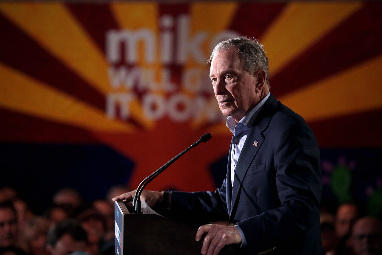
Spending a huge amount of resources without necessarily winning is exactly the kind of behavior that traditional theory has trouble explaining.

In traditional microeconomics, we often study how consumers maximize utility, how firms maximize profit, and how markets allocate resources through prices.

In real life, however, many forms of competition cannot be explained by the price mechanism alone. For example:

• Two firms spend money lobbying the government for an exclusive operating license
• Two political parties spend campaign resources to win an election
• Two companies spend on R&D to be the first to get a patent
• Two groups spend resources to win government subsidies or policy support

These cases have one thing in common: the players must spend costly resources, but the one who spends the most does not necessarily win.

Take elections as an example. A party that raises its campaign spending usually improves its chance of winning, but this does not mean the party that spends the most always wins.

We therefore need a theoretical model that describes how spending affects the chance of winning. This is exactly the question that contest theory sets out to answer.

From Rent-Seeking to Contests

One important source of contest theory is rent-seeking theory.

The rent in economics means economic rent, not the rent you pay for a house². Rent-seeking is the behavior of economic agents who spend resources to influence how a benefit is distributed, in order to obtain or keep that benefit.

Definition: Rent-seeking

The behavior of economic agents who spend resources competing with each other for the rents that government regulation of economic activity creates (Krueger, 1974, p. 291).

For example, the government is about to issue one exclusive business license worth 10 million dollars. Two firms both want it, so each hires consultants, lobbies policymakers, and devotes a lot of administrative and legal resources to it. Even if only one firm succeeds in the end, both firms have already paid the cost of competing.

This raises an important economic question:

A given benefit may be worth only 10 million dollars, but society may use up a large amount of extra resources just to decide who gets it.

If a traditional welfare analysis looks only at the deadweight loss from price distortions, it may underestimate the social cost of this kind of competition.

In The Welfare Costs of Tariffs, Monopolies, and Theft, Tullock (1967) stressed how important this kind of resource use is for welfare analysis. Krueger (1974) then developed the political economy of rent-seeking societies.

Efficient Rent Seeking by Tullock (1980) became a classic reference for probabilistic rent-seeking contest models. We can boil the research questions about Tullock contests down to three:

1. How does an individual’s spending determine the chance of winning?
2. How much will rational players spend?
3. Is the individually optimal outcome of the competition socially efficient?

The Basic Tullock Contest Model

Consider two players, $N$, who compete for one indivisible prize worth $V > 0$. Each player $i$ chooses an expenditure $x_i \in [0, \infty)$, which can stand for money, effort, time, or any other resource used in the competition.

To keep the analysis simple, assume that the cost of spending is linear, $C_i(x_i) = cx_i$, where $c \in R_{+}$ is the marginal cost of one unit of expenditure.

This post uses the following standard assumptions:

Variable	Assumption
Players	Two, $i = 1, 2$
Prize	A single indivisible prize worth $V$
Timing	Simultaneous moves
Information	Complete information
Strategy space	$x_i \geq 0$
Cost	$C_i(x_i) = cx_i$
Risk attitude	Risk neutral
Payment rule	Everyone pays their cost, whether they win or lose

The Contest Success Function

Next we need a function that describes how expenditure is turned into a chance of winning. It is called the contest success function (CSF). A common form of the CSF in Tullock contests is:

$$\begin{equation}\label{eq:general-csf} p_{i} (x_i,\cdots,x_n) = \dfrac{x_i^{r}}{\sum_{j = 1}^{n} x_{j}^{r}} \end{equation}$$

The symbols mean the following:

• $p_i$: the probability that player $i$ wins
• $x_i$: player $i$’s expenditure
• $x_j$: the opponent’s expenditure
• $r$: how strongly the outcome reflects differences in expenditure

Eq. $\eqref{eq:general-csf}$ is the most general form. This post considers only two players, so it can be rewritten as:

$$\begin{equation}\label{eq:two-contestor-csf} p_{i} (x_i, x_j) = \dfrac{x_i^{r}}{x_{i}^{r} + x_{j}^{r}} \end{equation}$$

When neither player spends anything, we usually define in addition that

$$p_1(0, 0) = p_2(0, 0) = \dfrac{1}{2}$$

that is, with no spending the winner is decided with equal probability³.

How Strongly the Outcome Depends on Spending

In the CSF, the parameter $r$ can be read as how sensitive the contest is to differences in expenditure. It measures how well the contest can tell strong players from weak ones.

A higher $r$ means that the result depends heavily on the players’ true ability or effort: a stronger or harder-working player has a much higher chance of winning. A lower $r$ means that the contest contains a lot of luck, random noise, or an imperfect judging process. In that case differences in ability are blurred, and everyone’s chance of winning is about the same even if their abilities differ.

To avoid complicated cases, this post uses only $r = 1$, so Eq. $\eqref{eq:two-contestor-csf}$ simplifies to

$$p_{i} (x_i, x_j) = \dfrac{x_i}{x_{i} + x_{j}}$$

Konrad (2009) and Corchón (2007) call this a lottery contest, so you can think of expenditure as the number of lottery tickets a player buys:

Example

Suppose player 1 spends 60 and player 2 spends 40. Then

$$\begin{aligned} p_{1} &= \dfrac{60}{60 + 40} = 0.6\\ p_{2} &= \dfrac{40}{60 + 40} = 0.4 \end{aligned}$$

Notice that this model measures relative spending, not absolute spending: if both players double their spending at the same time, their chances of winning stay exactly the same.

Payoff and Expected Payoff

Whether they win or lose, player $i$ has to pay the cost $cx_i$. So the payoff depends on the outcome of the contest:

• Win (with probability $p_i$): the player gets the prize $V$, and the payoff after cost is $V - cx_i$
• Lose (with probability $1 - p_i$): there is no prize, and the payoff is $-cx_i$

Because the outcome is random, a player cannot know in advance which case will happen. Multiplying each outcome by its probability and adding them up gives the expected payoff:

$$\underbrace{p_{i}(x_i, x_j)V}_{\text{expected prize}} - \underbrace{cx_{i}}_{\text{cost of spending}}$$

Under risk neutrality⁴, players care only about the expected payoff, so player $i$’s utility function can be written as:

$$\begin{equation}\label{eq:payoff} \pi_{i} (x_{i}, x_{j}) = \dfrac{x_{i}}{x_{i} + x_{j}} V - cx_{i} \end{equation}$$

Here $x_{i} + x_{j} > 0$, which means at least one player spends a positive amount (otherwise the winning probability is not defined). The more a player spends, the higher the chance of winning, but the higher the cost to pay as well. A rational player therefore does not raise spending without limit, but looks for the level that maximizes the expected payoff.

The Two-Player Symmetric Tullock Contest

With the expected payoff function, we can solve this game. Both players choose their spending at the same time, and each picks the level that maximizes their own expected payoff, given the opponent’s spending. When no player can raise their expected payoff by changing their spending alone, we have found a Nash equilibrium⁵.

The Individual Optimization Problem

For player $i$, the opponent’s spending $x_j$ is given, so the optimization problem is:

$$\max_{x_i \geq 0} \ \pi_i(x_i, x_j) = \dfrac{x_i}{x_i + x_j} V - cx_i$$

First consider $x_j > 0$. The derivative of the winning probability with respect to the player’s own spending is:

$$\dfrac{\partial}{\partial x_i} \left( \dfrac{x_i}{x_i + x_j} \right) = \dfrac{(x_i + x_j) - x_i}{(x_i + x_j)^2} = \dfrac{x_j}{(x_i + x_j)^2}$$

So the first partial derivative of the expected payoff with respect to $x_i$ is:

$$\dfrac{\partial \pi_i}{\partial x_i} = \underbrace{\dfrac{Vx_j}{(x_i + x_j)^2}}_{\text{marginal expected benefit}} - \underbrace{c}_{\text{marginal cost}}$$

When deciding whether to spend more, a player compares the marginal expected benefit of one more unit with its marginal cost:

• If the marginal expected benefit is larger than $c$, spending more raises the expected payoff
• If the marginal expected benefit is smaller than $c$, spending more is not worth it

An interior optimum must therefore satisfy the first-order condition (FOC):

$$\begin{equation}\label{eq:foc} \dfrac{Vx_j}{(x_i + x_j)^2} = c \end{equation}$$

The Second-Order Condition

The first-order condition only finds a candidate for the optimum, so we also need to check the second-order condition (SOC). Differentiating once more with respect to $x_i$:

$$\dfrac{\partial^2 \pi_i}{\partial x_i^2} = -\dfrac{2Vx_j}{(x_i + x_j)^3} < 0$$

Since $V > 0$ and $x_j > 0$, the expected payoff function is strictly concave in the player’s own spending. So whenever the solution of the first-order condition is positive, it is the unique optimal spending; if there is no positive solution, the optimum is the corner solution $x_i = 0$.

The Best Response Function

From Eq. $\eqref{eq:foc}$ we get:

$$(x_i + x_j)^2 = \dfrac{Vx_j}{c}$$

Spending is non-negative, so:

$$x_i + x_j = \sqrt{\dfrac{Vx_j}{c}}$$

Moving terms and adding the constraint $x_i \geq 0$ gives the best response function:

$$\begin{equation}\label{eq:br} BR_i(x_j) = \max \left\{ 0, \sqrt{\dfrac{Vx_j}{c}} - x_j \right\}, \quad x_j > 0 \end{equation}$$

It tells us how much player $i$ should spend, given how much the opponent spends.

Notice that when the opponent spends more, we do not always spend more too. Differentiating with respect to $x_j$ shows that $BR_i$ reaches its maximum at $x_j = \frac{V}{4c}$ and becomes zero beyond $x_j = \frac{V}{c}$:

• When the opponent spends little, spending a bit more pushes us to spend more as well, and the two are strategic complements
• When the opponent already spends a lot, chasing them is no longer worthwhile and we cut our spending instead, and the two become strategic substitutes

So the strategic relationship in a Tullock contest is neither always complementary nor always substitutive.

At $x_j = 0$, Eq. $\eqref{eq:br}$ cannot be applied directly. With the convention above that zero spending on both sides gives a tie, if the opponent spends nothing, any positive spending guarantees that we win, and the smaller it is the cheaper it is. But there is no smallest positive number, so there is no best response in this case. This boundary issue does not affect the positive-spending equilibrium below.

The Symmetric Nash Equilibrium

The two players have exactly the same valuation of the prize and the same cost function, so we first look for a symmetric equilibrium $x_1^* = x_2^* = x^*$. Substituting into Eq. $\eqref{eq:foc}$:

$$\dfrac{Vx^*}{(2x^*)^2} = \dfrac{V}{4x^*} = c$$

which gives:

$$\begin{equation}\label{eq:eq-input} x_1^* = x_2^* = \dfrac{V}{4c} \end{equation}$$

This is the equilibrium spending of the two-player symmetric lottery contest.

Theorem: Symmetric Nash equilibrium

In a Tullock contest with two players, complete information, simultaneous moves, the same prize valuation $V > 0$, the same linear cost $cx_i$, and $r = 1$, there is a unique pure-strategy Nash equilibrium:

$$(x_1^*, x_2^*) = \left( \dfrac{V}{4c}, \dfrac{V}{4c} \right)$$

Show proof

First consider the case where both players spend a positive amount. Their first-order conditions are:

$$\begin{aligned} \dfrac{Vx_2}{(x_1 + x_2)^2} &= c\\ \dfrac{Vx_1}{(x_1 + x_2)^2} &= c \end{aligned}$$

The denominators on the left are the same, so $x_1 = x_2$. In other words, any pure-strategy equilibrium with positive spending must be symmetric, and it is uniquely determined by Eq. $\eqref{eq:eq-input}$.

Next we rule out the boundary cases:

• If only one player spends a positive amount, for example $x_1 > 0 = x_2$, then player 1 wins with probability 1. They could halve their spending and still win for sure at a lower cost, so the original spending is not a best response
• If neither player spends anything, each player’s expected payoff is $\frac{V}{2}$. If either player switches to a small enough $\varepsilon > 0$, the winning probability becomes 1 and the expected payoff is $V - c\varepsilon > \frac{V}{2}$, so $(0, 0)$ is not an equilibrium

Finally we check that the candidate really is an equilibrium. When $x_j = \frac{V}{4c} > 0$, $\pi_i$ is strictly concave in $x_i$, and $x_i = \frac{V}{4c}$ satisfies the first-order condition, so it is the unique global maximum on $x_i \geq 0$, and $(x_1^*, x_2^*)$ is a Nash equilibrium. $\blacksquare$

Equilibrium Analysis

Once we have the equilibrium spending, we can go on to analyze the winning probability, the payoff, and the cost of the contest in equilibrium.

Equilibrium Winning Probability

Since equilibrium spending is equal:

$$p_1^* = p_2^* = \dfrac{x^*}{x^* + x^*} = \dfrac{1}{2}$$

Both players spend a positive amount of resources, and still each has only a half chance of winning. This is not a mistake in their decisions. Each knows that the opponent will adjust, so in the end they cancel out each other’s advantage.

Equilibrium Expected Payoff

Substituting the equilibrium spending back into Eq. $\eqref{eq:payoff}$:

$$\begin{equation}\label{eq:payoff-star} \pi_i^* = p_i^* V - cx_i^* = \dfrac{V}{2} - c \cdot \dfrac{V}{4c} = \dfrac{V}{4} \end{equation}$$

Each player’s equilibrium expected payoff is a quarter of the value of the prize.

Rent Dissipation

The total cost of spending by the two players is:

$$TC = \sum_{i=1}^{2} cx_i^* = 2c \cdot \dfrac{V}{4c} = \dfrac{V}{2}$$

We define the share of the total cost of the contest in the value of the prize as the rent dissipation rate:

$$\begin{equation}\label{eq:dissipation} D = \dfrac{\sum_{i} C_i(x_i^*)}{V} = \dfrac{1}{2} \end{equation}$$

In the standard two-player symmetric lottery contest, the players together spend resources worth 50% of the prize to compete for it. This answers the question at the start: even when everyone acts rationally, the competition itself still uses up a considerable amount of resources.

However, we should not treat all spending in contests as a loss of social welfare. If the spending has productive external benefits (for example in an R&D race), those benefits have to be included in the welfare analysis. Only when the spending is purely to win a given rent, and the cost stands for real resource use, can it be read as a corresponding waste of social resources.

Comparative Statics

Finally, let us look at how changing the parameters affects the equilibrium. From Eq. $\eqref{eq:eq-input}$, differentiate with respect to the value of the prize $V$ and the marginal cost $c$:

$$\begin{aligned} \dfrac{\partial x_i^*}{\partial V} &= \dfrac{1}{4c} > 0\\ \dfrac{\partial x_i^*}{\partial c} &= -\dfrac{V}{4c^2} < 0 \end{aligned}$$

The higher the value of the prize, the more players spend in equilibrium; the higher the marginal cost of spending, the less they spend.

When the cost rises, players cut their spending. Does the cost they actually pay fall too? Multiply the equilibrium spending by the unit cost $c$:

$$cx_i^* = c \cdot \dfrac{V}{4c} = \dfrac{V}{4}$$

The answer is no. When the cost per unit goes up, players reduce the quantity they spend, but the cost each player pays in equilibrium stays at $\frac{V}{4}$, whatever $c$ is. A higher $c$ makes each unit more expensive, but equilibrium spending $x_i^*$ falls in the same proportion, so the two exactly cancel out⁶.

Numerical Simulation

All the results so far are analytical solutions. In this section we check them in a different way: without using any formula, we compute the best responses numerically, then let the players respond to each other’s spending in turn, and repeat until nobody wants to change. The point we end at is the Nash equilibrium. Finally we compare it with the analytical solution.

The simulator below lets you change the parameters directly, and the results are computed in your browser in real time. You can also download the Python version of the code and run it yourself.

The horizontal axis of the figure is $x_1$ and the vertical axis is $x_2$. The solid line is player 1’s best response $x_1 = BR(x_2)$, and the dashed line is player 2’s best response $x_2 = BR(x_1)$. The point where the two lines cross is the Nash equilibrium, where neither player has an incentive to change their own spending alone.

Switch to the Expected payoff tab to see how player 1’s expected payoff $\pi_1(x_1, x_2^*)$ changes with their own spending $x_1$ when the opponent stays at the equilibrium spending $x_2^*$. The highest point of the curve falls exactly at $x_1^*$, which is the definition of a best response. Both figures can be downloaded as SVG, PNG, or PDF.

Try changing the parameters:

• With the default values $V = 100$, $c = 1$, $r = 1$, the intersection is at $(25, 25)$, which matches $\frac{V}{4c}$. The winning probability is $\frac{1}{2}$ and the rent dissipation rate is $\frac{1}{2}$.
• Whatever you do to $V$ or $c$, the numerical equilibrium always equals the value from the formula. When $c$ goes up, equilibrium spending goes down, but the rent dissipation rate stays at $\frac{1}{2}$. This matches the result of the previous section: the cost each player pays in equilibrium is always $\frac{V}{4}$.
• You can also move $r$ away from 1 and see how the picture changes⁷.

Conclusion

From the basic Tullock contest model, we get the following results:

What we analyze	Equilibrium result
Individual spending	$x_i^* = \frac{V}{4c}$
Individual winning probability	$p_i^* = \frac{1}{2}$
Individual expected payoff	$\pi_i^* = \frac{V}{4}$
Rent dissipation rate	$D = \frac{1}{2}$

Back to the three questions at the beginning: the first two are answered by the equilibrium spending and the equilibrium winning probability, and the third is given a basic measure by the rent dissipation rate.

These results rest on fairly strict assumptions: only two players, the same valuation and cost, simultaneous moves, complete information, and $r = 1$. So rather than memorizing the formulas, it is more worthwhile to remember the strategic logic behind them:

Whether a player should spend more depends not only on how large the prize is, but also on how much the opponent spends, and on how much more spending raises their own chance of winning.

When everyone tries to raise their chance of winning by spending more, rational individual decisions can together produce a considerable cost of competition. This is also why Tullock contests have become an important tool in rent-seeking theory (Krueger, 1974; Tullock, 1980), political competition, public choice, and the economics of conflict.

¹. This is the figure from the campaign’s final financial filings (Clark & Barrett, 2020). On the day he dropped out, CBS reported, based on data from the ad-tracking firm Kantar/CMAG, that his ad spending had already passed 570 million dollars (Ewall-Wice, 2020). The two numbers cover different scopes and dates, so they should not be compared directly. ↩

². Economic rent is the part of a factor’s earnings that exceeds what is needed to keep the factor in its current use. The idea goes back to Ricardo’s theory of land rent (Ricardo, 1817, chap. 2). ↩

³. This is a common convention. It affects only the boundary case where neither player spends anything, and it does not affect the positive-spending equilibrium below. ↩

⁴. If players are risk averse, what they maximize is expected utility rather than expected payoff, and equilibrium spending will differ. ↩

⁵. This post only discusses pure-strategy equilibria, in which each player chooses one level of spending with certainty. Randomized strategies are not considered. ↩

⁶. This conclusion depends on the assumptions of symmetry and linear cost, and it cannot be extended freely to other contest models. ↩

⁷. This goes beyond the model in this post, but it can still be observed. For $r \le 2$ the equilibrium stays symmetric, the numerical solution is $\frac{rV}{4c}$, and the rent dissipation rate is $\frac{r}{2}$. I do not derive this here; it is only an observation from the simulation. The simulator caps $r$ at 2, because for $r > 2$ the equilibrium expected payoff $\frac{(2-r)V}{4}$ is negative and no pure-strategy equilibrium exists. ↩

References

Clark, D., & Barrett, M. (2020, March 20). Bloomberg spent nearly $1 billion on his three-month presidential campaign. NBC News. https://www.nbcnews.com/politics/2020-election/bloomberg-spent-nearly-1-billion-his-three-month-presidential-campaign-n1165306

Corchón, L. C. (2007). The theory of contests: A survey. Review of Economic Design, 11(2), 69–100.

Ewall-Wice, S. (2020, March 4). How much did Mike Bloomberg spend per delegate? About $18 million. CBS News. https://www.cbsnews.com/news/bloomberg-delegate-18-million

Konrad, K. A. (2009). Strategy and dynamics in contests. Oxford University Press.

Krueger, A. O. (1974). The political economy of the rent-seeking society. American Economic Review, 64(3), 291–303. https://www.jstor.org/stable/1808883

Ricardo, D. (1817). On the principles of political economy and taxation. John Murray.

Tullock, G. (1967). The welfare costs of tariffs, monopolies, and theft. Western Economic Journal, 5(3), 224–232. https://doi.org/10.1111/j.1465-7295.1967.tb01923.x

Tullock, G. (1980). Efficient rent seeking. In J. M. Buchanan, R. D. Tollison, & G. Tullock (Eds.), Toward a theory of the rent-seeking society (pp. 97–112). Texas A&M University Press.