Overview
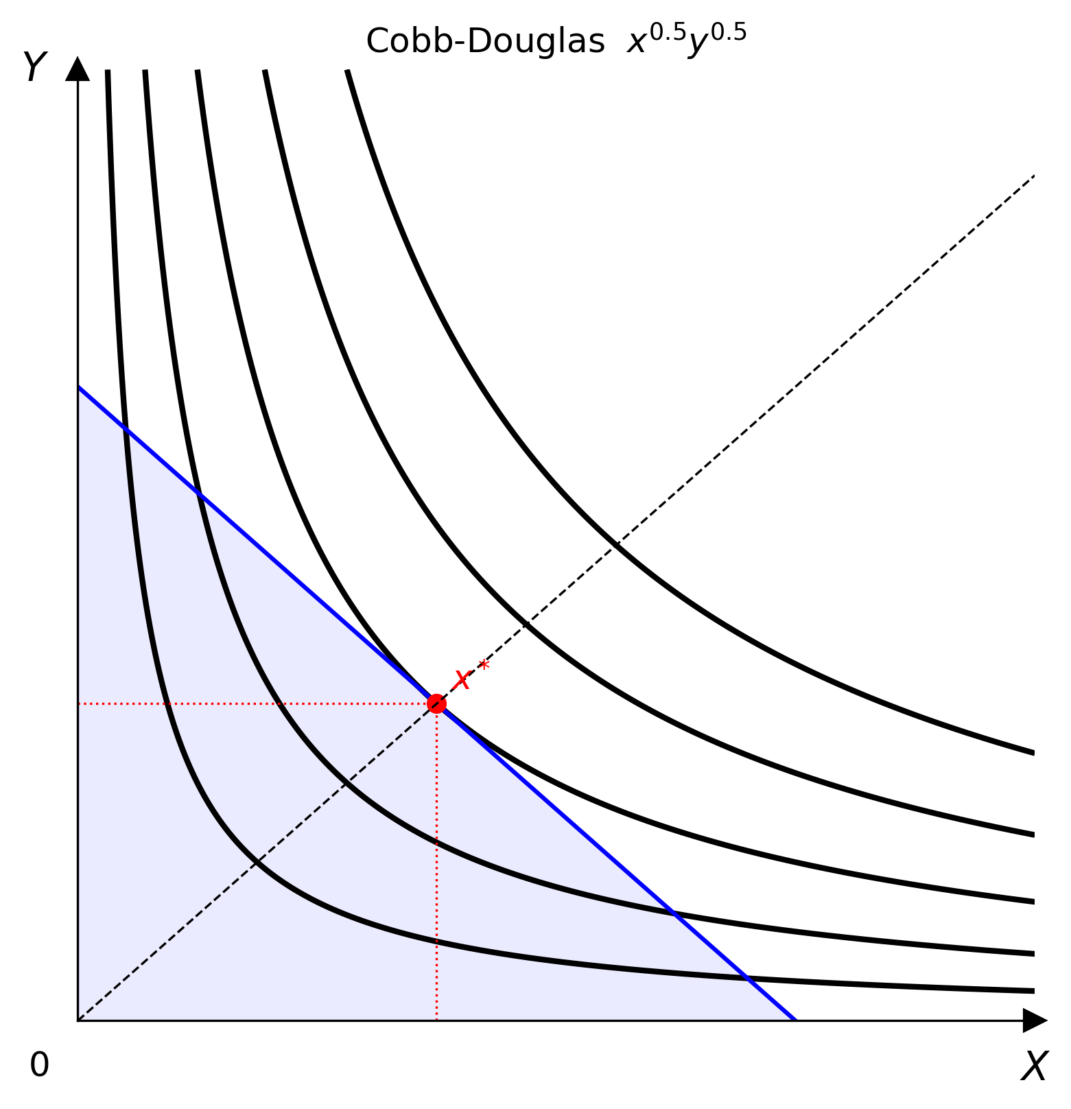
econ-viz is a Python package I built for drawing microeconomics teaching diagrams. Give it a utility function, prices, and income — it solves for the equilibrium, renders the indifference map and budget line, and exports to PNG, PDF, or SVG.
The motivation was straightforward: drawing these figures from scratch with matplotlib is tedious. Computing contour levels, finding tangency points, and formatting axes manually takes far longer than it should. I wanted a tool where I describe the model and let the library handle the rest.
Note
Current version: v1.4.0 · Test coverage: 99% · Tests: 235 passed
Features
Eight built-in utility models
Covering the full range of standard microeconomic preferences:
| Model | Class |
|---|---|
| Cobb-Douglas | CobbDouglas(alpha, beta) |
| Leontief (perfect complements) | Leontief(a, b) |
| Perfect Substitutes | PerfectSubstitutes(a, b) |
| CES | CES(alpha, rho) |
| Quasi-Linear | QuasiLinear(alpha) |
| Stone-Geary | StoneGeary(alpha, beta, x0, y0) |
| Translog | Translog(alpha, beta, gamma) |
| Satiation | Satiation(x_sat, y_sat) |
Automatic equilibrium solving
solve() uses SLSQP and handles interior solutions, corner solutions, and Leontief kink optima. It returns a structured Equilibrium object with fields x, y, utility, and bundle_type.
Analysis tools
comparative_statics()— numerical estimation of the six Marshallian demand partial derivativesslutsky_matrix()— two-good Slutsky substitution matrix with symmetry and negative-semidefiniteness checksHomogeneityAnalyzer— homogeneity degree, Euler theorem residual, homotheticity, and degree-0 demand checks
Multi-panel figures
Figure with Layout enum (side-by-side, stacked, grid) composes multiple Canvas panels into a single figure — ideal for before/after price-change comparisons.
Demand diagrams
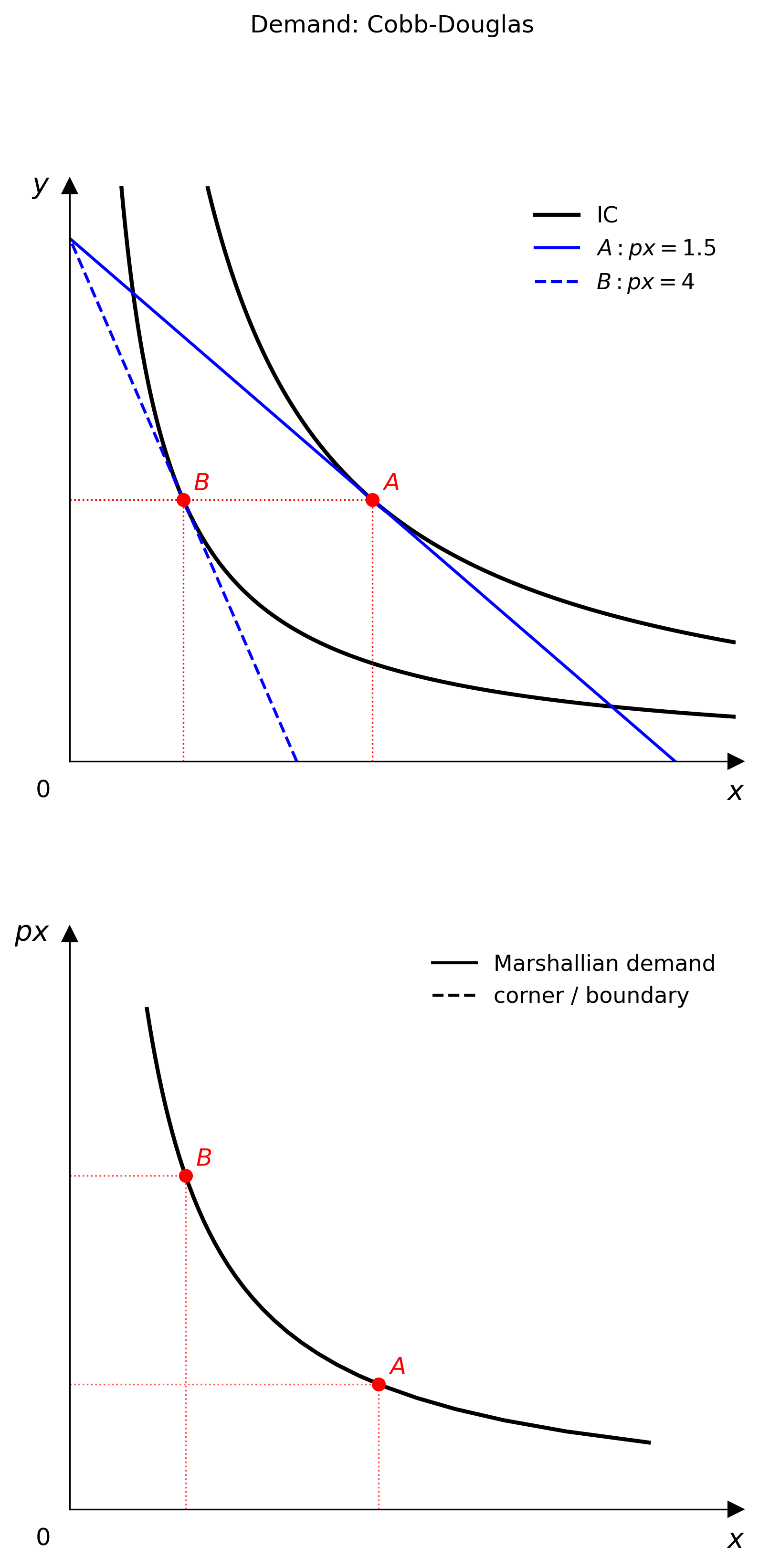
PricePath / IncomePath + DemandDiagram link the goods-space equilibrium locus to the Marshallian demand curve. Generates PCC and ICC teaching diagrams automatically.
LaTeX parser
Pass a LaTeX expression such as x^{0.4} y^{0.6} directly and get back a fully configured model instance.
Animation
Animator supports parameter sweeps, price sweeps, and income sweeps, exporting as GIF — useful for lecture slides and interactive documentation.
Notebook widgets
WidgetViewer in Jupyter adds a slider plus numeric input for each model parameter, so you can drag or type exact values and watch the equilibrium update live.
Installation
1 | pip install econ-viz |
Requires Python 3.10 or later. Dependencies: numpy, matplotlib, scipy, sympy.
Quick Start
Minimal example
1 | from econ_viz import Canvas, levels, solve |
LaTeX parser
1 | from econ_viz import parse_latex, Canvas, levels, solve |
Demand diagram
1 | from econ_viz import DemandDiagram, LinearBudget, PricePath |
Slutsky matrix
1 | from econ_viz import slutsky_matrix |
Edgeworth Box
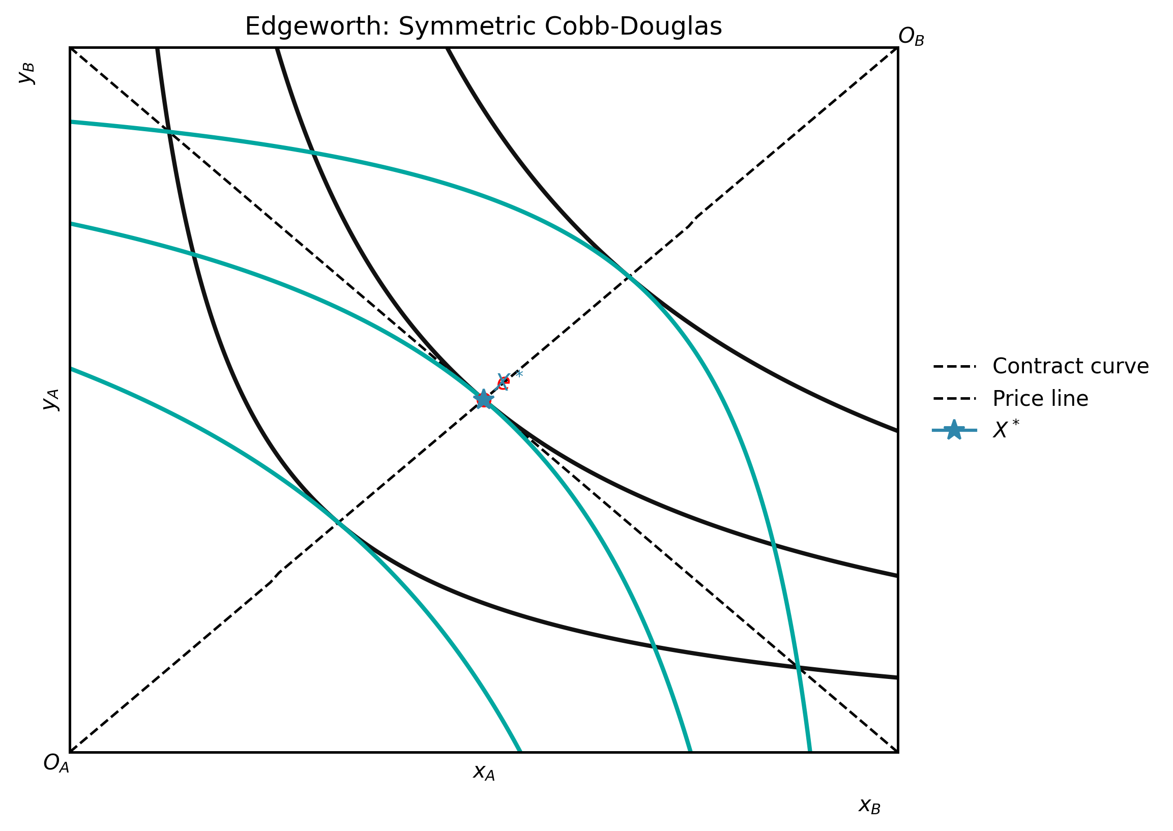
1 | from econ_viz import EdgeworthBox, EquilibriumFocusConfig |
CLI
1 | # List all supported models |