佇列 (queue) 的應用比堆疊更廣泛,也相較於堆疊稍微複雜一點。

定義:佇列 (queue)

佇列是一種動態集合,其中元素的插入與刪除遵循先進先出 (first-in-first-out, FIFO) 的原則,每次刪除的元素,永遠是目前集合中最早被插入、且尚未被刪除的那一個。

佇列支援兩種基本操作:

  • enqueue(Q, x):將元素 $x$ 插入佇列 $Q$ 的尾端 (tail)
  • dequeue(Q):刪除並回傳佇列 $Q$ 頭端 (head) 的元素

基本操作

不同於堆疊,佇列的操作分別在頭尾兩端,新增元素從尾端放進去,要拿元素僅能從頭端拿走。

佇列的操作分為:將元素放到尾端的入列 (enqueue)、將頭端元素拿掉的出列 (dequeue),以及查看頭端但不動它的查佇列首 (front)

但比較需要注意的是,如果我們使用堆疊的方法處裡入/出列,會發生如圖 1 的問題:
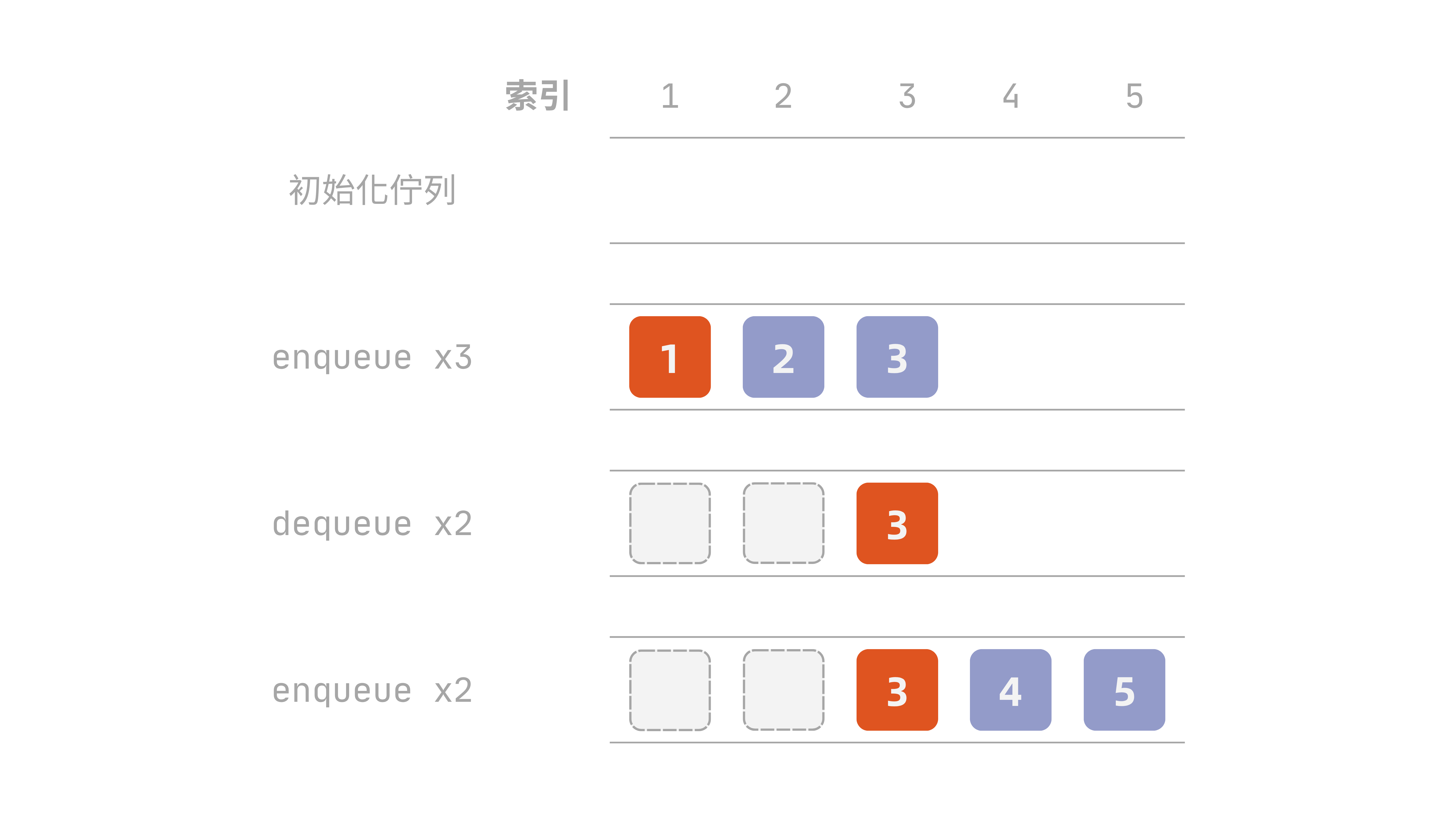
佇列指標漂移示意圖
圖 1:佇列指標漂移示意圖

最後一步的 tail 跑到 6,已經超出陣列範圍,但佇列裡其實只有 3 個元素,前面還空著 2 格——空間沒用完卻已塞不下了。

因此通常我們會使用環形佇列 (circular queue) 的技巧,將指標繞一圈,在邏輯上形成一個環,重複利用。

入列

入列首先要檢查佇列是否已滿,並且執行以下操作:

  • 若已滿:拒絕插入,可回傳/輸出失敗訊息
  • 若未滿:將元素放進 tail 指到的那一格,再把 tail 往後移一格;若 tail 已經在最後一格,則繞回第一格
1
2
3
4
5
6
7
8
9
10
11
Enqueue(Q, x)
if (tail[Q] mod length[Q]) + 1 = head[Q] then
error "overflow"
else
Q[tail[Q]] = x
if tail[Q] = length[Q] then
tail[Q] = 1
else
tail[Q] = tail[Q] + 1
end if
end if

這裡的 (tail[Q] mod length[Q]) + 1 就是「tail 的下一格」,寫成 mod 是為了處理繞回開頭的情況。如果下一格剛好就是 head,代表再放就會撞上頭端,因此判定為已滿。

為什麼長度 $n$ 的陣列只能裝 $n-1$ 個元素?

注意上面的判定式:head[Q] = tail[Q]滿卻是tail 的下一格等於 head,也就是刻意留了一格不用。原因是這兩個狀態會撞在一起。假設真的把 $n$ 格全部塞滿的話,tail 從最後一格繞回開頭之後,剛好會停在 head 的位置,於是 head[Q] = tail[Q]——但這正是佇列為空的判定條件。同一組指標值同時代表空與滿,程式就再也分不出來了。

因此環形佇列會犧牲一格當作分隔,讓 head[Q] = tail[Q] 唯一對應空這個狀態,長度 $n$ 的陣列實際可用容量是 $n-1$。若真的需要用滿 $n$ 格,就得額外維護一個 size 欄位記錄目前元素個數,改用 size = 0 判空、size = length[Q] 判滿,不再依賴指標關係。

出列

出列就是判斷是否為空:

  • 若為空:拒絕出列,可回傳/輸出失敗訊息
  • 若非空:取出 head 指到的元素,將 head 往後移一格(同樣會繞回開頭),回傳該元素

用虛擬碼的方式撰寫如下:

1
2
3
4
5
6
7
8
9
10
11
12
Dequeue(Q)
if head[Q] = tail[Q] then
error "underflow"
else
x = Q[head[Q]]
if head[Q] = length[Q] then
head[Q] = 1
else
head[Q] = head[Q] + 1
end if
return x
end if

查佇列首

查佇列首則是一樣先判斷是否為空:

  • 若為空:拒絕查看,可回傳/輸出失敗訊息
  • 若非空:回傳頭端元素,但不將其移除

用虛擬碼的方式撰寫如下:

1
2
3
4
5
6
Front(Q)
if head[Q] = tail[Q] then
error "underflow"
else
return Q[head[Q]]
end if

各項操作時間複雜度

enqueuedequeuefront 三個操作都只碰 head[Q]tail[Q] 這兩個指標,以及它們指到的那一格——不管是判斷、讀寫,還是移動指標(包含繞回開頭的 mod 運算),動作次數都是固定的,完全不需要因為佇列裡目前有幾個元素而多做事,所以都是 $O(1)$。

操作 時間複雜度
enqueue $O(1)$
dequeue $O(1)$
front $O(1)$
走訪(訪問所有元素) $O(n)$

這裡要特別留意的是,環形佇列的 $O(1)$ 是繞回開頭換來的。如果不繞、改成每次 dequeue 就把後面的元素整批往前搬一格來補上空位,head 確實永遠會停在第一格,但每次出列都要搬動 $O(n)$ 個元素,佇列最核心的操作就從 $O(1)$ 掉到 $O(n)$ 了。

同堆疊一樣,走訪整個佇列一樣不算標準操作,佇列僅保證能碰到 head。如果想看過每一個元素,只能從 head 開始一路往後,沒有辦法跳著存取,每個元素都要碰一次,因此是 $O(n)$;用 dequeue 走訪還會把佇列本身清空,除非邊 dequeue 邊存到別的地方再 enqueue 回去。

佇列實作

使用陣列

以下用固定大小的陣列實作環形佇列,其中 size() 的寫法利用了 Python % 運算子的一個特性1

1
2
3
4
5
6
7
8
9
10
11
12
13
14
15
16
17
18
19
20
21
22
23
24
25
26
27
28
29
30
31
32
33
34
35
36
37
38
39
40
41
42
43
44
45
46
47
48
49
50
class ArrayQueue:
def __init__(self, capacity: int):
"""初始化佇列"""
self.capacity: int = capacity
self._queue: list[int] = [0] * self.capacity
self._head: int = 0
self._tail: int = 0

def is_empty(self) -> bool:
"""檢查佇列是否為空"""
return self._head == self._tail

def size(self) -> int:
"""回傳佇列長度"""
return (self._tail - self._head) % self.capacity

def _next(self, endpoint: int) -> int:
"""回傳某索引下一格"""
return (endpoint + 1) % self.capacity

def enqueue(self, x: int) -> None:
"""入列"""
if self._next(self._tail) == self._head:
raise IndexError("佇列已滿")
self._queue[self._tail] = x
self._tail = self._next(self._tail)

def dequeue(self) -> int:
"""出列"""
if self.is_empty():
raise IndexError("佇列為空")
x = self._queue[self._head]
self._head = self._next(self._head)
return x

def front(self) -> int:
"""查看佇列首"""
if self.is_empty():
raise IndexError("佇列為空")
return self._queue[self._head]

def __repr__(self) -> str:
"""轉為字串"""
result: list[str] = []
curr_idx = self._head
while curr_idx != self._tail:
result.append(str(self._queue[curr_idx]))
curr_idx = self._next(curr_idx)

return " <- ".join(result)

使用鏈結串列

首先定義節點:

1
2
3
4
class ListNode:
def __init__(self, data: int):
self.data: int = data
self.next: ListNode | None = None

接著開始實作:

1
2
3
4
5
6
7
8
9
10
11
12
13
14
15
16
17
18
19
20
21
22
23
24
25
26
27
28
29
30
31
32
33
34
35
36
37
38
39
40
41
42
43
44
45
46
47
48
49
50
51
52
53
54
55
56
57
58
class LinkedListQueue:
def __init__(self):
"""初始化佇列"""
self._head: ListNode | None = None
self._tail: ListNode | None = None
self._size: int = 0

def is_empty(self) -> bool:
"""檢查佇列是否為空"""
return not self._head

def size(self) -> int:
"""回傳佇列長度"""
return self._size

def enqueue(self, x: int) -> None:
"""入列"""
node: ListNode = ListNode(x)
if self.is_empty():
self._head = node
self._tail = node
else:
self._tail.next = node
self._tail = node
self._size += 1

def dequeue(self) -> int:
"""出列"""
if self.is_empty():
raise IndexError("佇列為空")

node = self._head
self._head = self._head.next
if self._head is None:
self._tail = None

self._size -= 1
return node.data

def front(self) -> int:
"""查佇列首"""
if self.is_empty():
raise IndexError("佇列為空")
return self._head.data

def __repr__(self) -> str:
"""轉為字串"""
if self.is_empty():
return ""

result: list[str] = []
curr = self._head

while curr:
result.append(str(curr.data))
curr = curr.next

return " <- ".join(result)

雙向佇列

前面實作的佇列限制得很死,佇列只能從尾端進、頭端出。這個限制換來的是 $O(1)$ 的操作,但也讓某些需求做不到——例如想反悔剛才放進去的元素,或是想從隊伍最後面插隊。

雙向佇列 (double-ended queue, deque) 放寬了這個限制:頭尾兩端都可以進、也都可以出,且四個操作的時間複雜度全部都是 $O(1)$。

定義:雙向佇列 (deque)

雙向佇列是一種同時具備堆疊與佇列性質的動態集合,其兩端皆可執行插入與刪除操作。

放寬限制之後,它同時涵蓋了前面學過的兩種結構:只從尾端進、頭端出,它就是佇列;只從尾端進、尾端出,它就是堆疊。因此雙向佇列可以視為堆疊與佇列的一般化形式。

基本操作

兩端都能進出,因此操作數量是普通佇列的兩倍:

方法名 描述 時間複雜度
push_first() 將元素新增至佇首 $O(1)$
push_last() 將元素新增至佇尾 $O(1)$
pop_first() 刪除佇首元素 $O(1)$
pop_last() 刪除佇尾元素 $O(1)$
peek_first() 訪問佇首元素 $O(1)$
peek_last() 訪問佇尾元素 $O(1)$

上面是通用的命名,實際在 Python 中會對應到 collectionsdeque 的方法(以下 d 為一個 deque 物件):

方法名 deque 本篇的佇列
push_last() d.append(x) enqueue(x)
push_first() d.appendleft(x) ——
pop_first() d.popleft() dequeue()
pop_last() d.pop() ——
peek_first() d[0] front()
peek_last() d[-1] ——

最右欄空著的四格就是雙向佇列多出來的能力。只用 push_last()pop_first() 就是普通佇列;只用 push_last()pop_last()(兩個都在佇尾)就是堆疊——這也是為什麼一個 deque 就能同時扮演堆疊與佇列。

另外要注意,deque 雖然可以用索引存取中間的元素,但那是 $O(n)$:它不是陣列,越靠近中間就要走越多步。**需要頻繁隨機存取就別用 deque 而是 list

使用陣列

1
2
3
4
5
6
7
8
9
10
11
12
13
14
15
16
17
18
19
20
21
22
23
24
25
26
27
28
29
30
31
32
33
34
35
36
37
38
39
40
41
42
43
44
45
46
47
48
49
50
51
52
53
54
55
56
57
58
59
60
61
62
63
64
65
66
67
68
69
70
71
72
73
74
75
class ArrayDeque:
def __init__(self, capacity: int):
"""初始化雙向佇列"""
self.capacity: int = capacity
self._deque: list[int] = [0] * self.capacity
self._head: int = 0
self._tail: int = 0

def is_empty(self) -> bool:
"""檢查佇列是否為空"""
return self._head == self._tail

def size(self) -> int:
"""回傳佇列長度"""
return (self._tail - self._head) % self.capacity

def _next(self, endpoint: int) -> int:
"""回傳某索引下一格"""
return (endpoint + 1) % self.capacity

def _prev(self, endpoint: int) -> int:
"""回傳某索引前一格"""
return (endpoint - 1) % self.capacity

def push_last(self, x: int) -> None:
"""入列——尾端"""
if self._next(self._tail) == self._head:
raise IndexError("佇列已滿")
self._deque[self._tail] = x
self._tail = self._next(self._tail)

def push_first(self, x: int) -> None:
"""入列——頭端"""
if self._next(self._tail) == self._head:
raise IndexError("佇列已滿")
self._head = self._prev(self._head)
self._deque[self._head] = x

def pop_last(self) -> int:
"""出列——尾端"""
if self.is_empty():
raise IndexError("佇列為空")
self._tail = self._prev(self._tail)
x = self._deque[self._tail]
return x

def pop_first(self) -> int:
"""出列——頭端"""
if self.is_empty():
raise IndexError("佇列為空")
x = self._deque[self._head]
self._head = self._next(self._head)
return x

def peek_last(self) -> int:
"""查看佇列尾"""
if self.is_empty():
raise IndexError("佇列為空")
return self._deque[self._prev(self._tail)]

def peek_first(self) -> int:
"""查看佇列首"""
if self.is_empty():
raise IndexError("佇列為空")
return self._deque[self._head]

def __repr__(self) -> str:
"""轉為字串"""
result: list[str] = []
curr_idx = self._head
while curr_idx != self._tail:
result.append(str(self._deque[curr_idx]))
curr_idx = self._next(curr_idx)

return " <- ".join(result)

使用鏈結串列

首先定義節點。與前面佇列的單向節點不同,這裡的節點必須同時記住前後兩個方向2

1
2
3
4
5
class DoublyListNode:
def __init__(self, data: int):
self.data: int = data
self.prev: DoublyListNode | None = None
self.next: DoublyListNode | None = None

與陣列實作雙向佇列的方式,以下用鏈結串列實作:

1
2
3
4
5
6
7
8
9
10
11
12
13
14
15
16
17
18
19
20
21
22
23
24
25
26
27
28
29
30
31
32
33
34
35
36
37
38
39
40
41
42
43
44
45
46
47
48
49
50
51
52
53
54
55
56
57
58
59
60
61
62
63
64
65
66
67
68
69
70
71
72
73
74
75
76
77
78
79
80
81
82
83
84
85
86
87
88
89
90
91
92
93
94
class LinkedListDeque:
def __init__(self):
"""初始化佇列"""
self._head: DoublyListNode | None = None
self._tail: DoublyListNode | None = None
self._size: int = 0

def is_empty(self) -> bool:
"""檢查佇列是否為空"""
return not self._head

def size(self) -> int:
"""回傳佇列長度"""
return self._size

def push_last(self, x: int) -> None:
"""入列——尾端"""
node: DoublyListNode = DoublyListNode(x)
if self.is_empty():
self._head = node
self._tail = node
else:
self._tail.next = node
node.prev = self._tail
self._tail = node
self._size += 1

def push_first(self, x: int) -> None:
"""入列——頭端"""
node: DoublyListNode = DoublyListNode(x)
if self.is_empty():
self._head = node
self._tail = node
else:
self._head.prev = node
node.next = self._head
self._head = node
self._size += 1

def pop_first(self) -> int:
"""出列——頭端"""
if self.is_empty():
raise IndexError("佇列為空")

node = self._head
self._head = self._head.next
if self._head is None:
self._tail = None
else:
self._head.prev = None

self._size -= 1
return node.data

def pop_last(self) -> int:
"""出列——尾端"""
if self.is_empty():
raise IndexError("佇列為空")

node = self._tail
self._tail = self._tail.prev
if self._tail is None:
self._head = None
else:
self._tail.next = None

self._size -= 1
return node.data

def peek_first(self) -> int:
"""查佇列首"""
if self.is_empty():
raise IndexError("佇列為空")
return self._head.data

def peek_last(self) -> int:
"""查佇列尾"""
if self.is_empty():
raise IndexError("佇列為空")
return self._tail.data

def __repr__(self) -> str:
"""轉為字串"""
if self.is_empty():
return ""

result: list[str] = []
curr = self._head

while curr:
result.append(str(curr.data))
curr = curr.next

return " <- ".join(result)

使用 deque

前面使用陣列與鏈結串列實作佇列,雖然可以了解底層邏輯,但實務上鮮少人這麼做,理由很簡單——太麻煩了!而如果偷懶直接拿 Python 的 list 當佇列用(append 進、pop(0) 出),效能又會非常慘:

元素個數 list.pop(0) deque.popleft() 倍數
10,000 6.0 ms 0.3 ms 18x
50,000 195.0 ms 1.6 ms 124x
100,000 781.8 ms 3.3 ms 240x
200,000 3894.0 ms 8.0 ms 488x

慢的原因就是前面提到的:pop(0) 會把後面所有元素往前搬一格來補上空位,每次出列都是 $O(n)$。

通常來說,若要使用佇列,會利用 Python 內建函式庫的 collections 裡的 deque3

deque 位於 collections 模組中,並非內建型別,因此使用前必須先匯入:

1
from collections import deque

deque 有三種常見的建立方式:

1
2
3
d = deque()             # 建立空雙向佇列
d = deque([1, 2, 3]) # 從可迭代物件建立雙向佇列
d = deque(range(1, 5)) # 同上

接著是四個端點操作,與前面自己實作的方法逐一對應:

1
2
3
4
5
6
7
8
9
10
11
12
d = deque([1, 2, 3])

d.append(4) # 入列至佇尾
d.appendleft(0) # 入列至佇首

d[0] # 查看佇首
d[-1] # 查看佇尾

d.pop() # 從佇尾出列
d.popleft() # 從佇首出列

len(d) # 目前元素個數

命名規則相當好記:沒有 left 的都在尾端appendpop),與 list 的用法一致;加上 left 的則在頭端appendleftpopleft)。

因此把 deque 當作佇列使用時,進出只會用到 appendpopleft

1
2
3
4
q = deque()
q.append(x) # 入列
q.popleft() # 出列
q[0] # 查佇列首

當作堆疊使用則是 append 搭配 pop,兩者都在尾端,寫法與 list 完全相同。

若對空的 deque 執行出列或查看,會拋出 IndexError,與前面自己實作時 raise IndexError 的行為一致:

1
2
3
deque().pop()      # IndexError: pop from an empty deque
deque().popleft() # IndexError: pop from an empty deque
deque()[0] # IndexError: deque index out of range

實務上判斷是否為空,直接寫 if not d: 即可。

除了上述基本操作外,deque 建立時還可以指定 maxlen,也就是容量上限:

1
d = deque(maxlen=3)

指定之後,一旦元素數量達到上限,再放入新元素時另一端最舊的元素會自動被擠掉,既不會拋出例外,也不需要自己處理:

1
2
3
4
5
append(1)  ->  deque([1])
append(2) -> deque([1, 2])
append(3) -> deque([1, 2, 3])
append(4) -> deque([2, 3, 4]) # 1 被擠掉
append(5) -> deque([3, 4, 5]) # 2 被擠掉

方向是相對的:從佇尾放入,擠掉的是佇首;從佇首放入(appendleft),擠掉的則是佇尾——永遠從另一端推出去。

滿了要報錯,還是丟掉最舊的?

可以很明顯地注意到 dequemaxlen 與前面自己實作的 ArrayDeque 行為並不相同:前者認為滿了代表出事,應該讓呼叫端知道,滿了會 raise IndexError("佇列已滿");後者則是只在乎最近的 $N$ 筆,舊的本來就該淘汰

maxlen 的用途可理解為僅保留最近 $N$ 筆資料。常見的情境包括保留最近若干筆日誌、記錄使用者最近幾次操作以支援復原,以及滑動視窗——視窗往前移動時新元素進入、最舊的元素自動離開等。

若沒有 maxlen,同樣的效果得自己手動維護:

1
2
3
d.append(x)
if len(d) > 3:
d.popleft()

值得注意的是,d.maxlen 為唯讀屬性,建立之後無法更改;未指定時則代表沒有上限。

複雜度比較

接著我們使用以下表格來比較兩種實作佇列的差異:

陣列佇列(ArrayQueue 鏈結串列佇列(LinkedListQueue collections.deque
容量 建立時就固定,且實際可用只有 $n-1$ 理論上無上限(僅受記憶體限制) 預設無上限,可用 maxlen 指定
需要事先知道大小
額外空間開銷 一開始就配置整個陣列,沒裝滿的格子也一直佔著 每個節點多一個 next 指標的空間 指標開銷分攤到整個區塊上
記憶體局部性 好,元素連續存放,快取命中率高 差,節點散落在記憶體各處 好,區塊內部連續存放
enqueue / dequeue / front 均 $O(1)$ 均 $O(1)$ 均 $O(1)$

三個核心操作的時間複雜度完全一樣,差別在記憶體怎麼用。陣列版在建立時就把 $n$ 格配置好,之後不管實際裝幾個,那塊空間都佔著;鏈結串列版則是有幾個元素就配置幾個節點,但每個節點都要多存一個 next 指標。

同堆疊一樣,實際跑起來陣列版通常比較快。元素在記憶體裡連續排列,讀寫時記憶體局部性較好、快取命中率較高;鏈結串列版每個節點的位置是分散的,即使操作次數相同,實際存取速度仍會慢一截。

至於自己實作時怎麼選,關鍵在於事先知不知道會有多少元素

  • 上限明確、又在意速度(例如固定大小的緩衝區):用陣列版
  • 完全不知道會來多少(例如 BFS 的待處理節點):用鏈結串列版,不必煩惱滿了要怎麼辦

不過實務上兩者都不必自己寫。deque 的內部結構是一串固定大小的區塊,再以雙向指標串接起來——區塊內部連續存放,因此保有陣列的記憶體局部性;區塊之間用指標相連,因此長度不受限制,而且指標的開銷是分攤在整個區塊上,而不是每個元素各付一次。換句話說,它同時拿下了上表前兩欄的優點,這也是為什麼標準函式庫值得直接拿來用。

雙向佇列的兩種實作也是同樣的取捨,但有兩個佇列沒有的差異:

陣列雙向佇列(ArrayDeque 鏈結串列雙向佇列(LinkedListDeque
容量 建立時就固定,且實際可用只有 $n-1$ 理論上無上限(僅受記憶體限制)
每個元素的額外空間 兩個指標(prevnext
佇尾的位置 _tail 指向空格,取值需再算一次 _prev() _tail 直接指向節點
六項操作 均 $O(1)$ 均 $O(1)$

第一個差異是空間:佇列的鏈結串列版每個節點只多存一個 next,雙向佇列則要存 prevnext 兩個,額外開銷加倍。這是換取「兩端都能 $O(1)$ 進出」所付出的代價——單向串列刪除佇尾必須先找到前一個節點,只能從頭走一遍,是 $O(n)$。

第二個差異是取值的便利性。陣列版沿用佇列的慣例,_head 指向第一個元素、_tail 指向下一個空格,兩個指標的語意並不對稱,因此 peek_last() 要多算一次 _prev(_tail) 才拿得到佇尾;鏈結串列版的 _tail 直接就是最後一個節點,peek_first()peek_last() 完全對稱。

這個不對稱也決定了陣列版四個進出操作的寫法,實作時特別容易寫反:

操作 指標指向 順序
push_last _tail 為空格 先寫入,再移動指標
pop_last _tail 為空格 先移動指標,再讀取
push_first _head 為元素 先移動指標,再寫入
pop_first _head 為元素 先讀取,再移動指標

規則是:指標指向空格時「先寫後移、先移後讀」,指向元素時則完全相反。

鏈結串列版沒有這個問題,但有另一個要注意的地方:雙向串列的每條連結都是成對的,接上新節點時要同時設定兩個方向,移除節點時也要把兩邊都斷乾淨。撰寫頭端與尾端的鏡像版本時,_head_tailprevnext 必須同時對調,只換其中一組就會把串列接錯。

實作

LeetCode 933:最近的請求次數

題目敘述

寫一個 RecentCounter 類別,用於計算最近 3000 毫秒內的請求次數。請實作以下方法:

  • RecentCounter():初始化計數器,請求數為 0
  • int ping(int t):在時間 t 加入一個新請求,回傳發生在 [t - 3000, t] 範圍內的請求總數(包含新加入的這一個)

保證每次呼叫 ping 時傳入的 t 都比前一次更大。

範例

1
2
3
4
5
6
7
8
9
10
11
12
13
輸入:
["RecentCounter", "ping", "ping", "ping", "ping"]
[[], [1], [100], [3001], [3002]]
輸出:
[null, 1, 2, 3, 3]

解釋:
recentCounter = RecentCounter()
recentCounter.ping(1) # 請求 = [1],範圍 [-2999, 1],回傳 1
recentCounter.ping(100) # 請求 = [1, 100],範圍 [-2900, 100],回傳 2
recentCounter.ping(3001) # 請求 = [1, 100, 3001],範圍 [1, 3001],回傳 3
recentCounter.ping(3002) # 請求 = [1, 100, 3001, 3002],範圍 [2, 3002],回傳 3
# 此時 1 已經掉出範圍

新的請求一律加入佇尾;接著只要佇首的時間早於 t - 3000,就代表它已經掉出範圍,從佇首移除。由於題目保證 t 遞增,範圍的左邊界只會往右移,掉出去的請求永遠不會再回來,因此可以安心直接丟棄,最後佇列裡剩下的就是範圍內的所有請求,數量即為答案:

1
2
3
4
5
6
7
8
9
10
11
from collections import deque

class RecentCounter:
def __init__(self):
self.q = deque()

def ping(self, t: int) -> int:
self.q.append(t)
while self.q[0] < t - 3000:
self.q.popleft()
return len(self.q)

要注意這裡必須使用 while 而非 if——單次 ping 需要淘汰的請求數量並不固定,取決於這次的 t 跳了多遠。以 ping(1)ping(2)ping(3) 之後接著 ping(5000) 為例,範圍變成 [2000, 5000],前三個請求會一次全部掉出範圍。

複雜度方面,單次 ping 最壞情況為 $O(n)$(一次淘汰所有既有請求),但每個請求終其一生只會被加入一次、移除一次,因此 $n$ 次 ping 的總成本是 $O(n)$,攤銷後每次為 $O(1)$

題目條件與使用結構

本題之所以適合佇列,是三個條件湊在一起的結果:t 遞增,所以新請求直接加到佇尾即可,不必排序或搜尋;範圍左邊界只往右移,所以掉出去的請求可以直接丟棄;題目只問「有幾個」而不問「是哪些」,所以 len() 就是答案。先進先出、只碰兩端——正適合使用佇列。

LeetCode 232:用堆疊實作佇列

題目敘述

僅使用兩個堆疊,實作一個先進先出的佇列。這個佇列必須支援一般佇列的所有操作(pushpoppeekempty)。實作 MyQueue 類別:

  • void push(int x):將元素 x 推入佇列尾端
  • int pop():從佇列頭端移除並回傳元素
  • int peek():回傳佇列頭端的元素
  • boolean empty():若佇列為空則回傳 true,否則回傳 false

僅能使用堆疊的標準操作,也就是推入頂端、查看/彈出頂端、判斷是否為空。

範例

1
2
3
4
5
6
7
8
9
10
11
12
13
輸入:
["MyQueue", "push", "push", "peek", "pop", "empty"]
[[], [1], [2], [], [], []]
輸出:
[null, null, null, 1, 1, false]

解釋:
myQueue = MyQueue()
myQueue.push(1) # queue = [1]
myQueue.push(2) # queue = [1, 2]
myQueue.peek() # 回傳 1
myQueue.pop() # 回傳 1,queue = [2]
myQueue.empty() # 回傳 False

一個堆疊會把元素的順序顛倒過來,那麼顛倒兩次,順序就轉回來了。因此準備兩個堆疊:push 進來的元素一律放進 _in,而 poppeek 一律從 _out 取;當 _out 空了,就把 _in 裡的元素整批倒過去,順序自然就是先進先出:

1
2
push 1, 2, 3       _in  = [1, 2, 3]        頂端在右,pop 會先拿到 3
整批倒進 _out _out = [3, 2, 1] pop 會先拿到 1,正是先進先出

由於 poppeek 都需要這個動作,把它抽成一個私有方法:

1
2
3
4
5
6
7
8
9
10
11
12
13
14
15
16
17
18
19
20
21
22
23
class MyQueue:
def __init__(self):
self._in: list[int] = []
self._out: list[int] = []

def push(self, x: int) -> None:
self._in.append(x)

def _transfer(self) -> None:
if not self._out:
while self._in:
self._out.append(self._in.pop())

def pop(self) -> int:
self._transfer()
return self._out.pop()

def peek(self) -> int:
self._transfer()
return self._out[-1]

def empty(self) -> bool:
return len(self._in) == 0 and len(self._out) == 0

這裡有兩個地方特別容易寫錯。第一是 _transfer 的判斷式:必須等 _out 完全空了才能倒。若 _out 還有元素在等待就把 _in 倒過去,新元素會疊在舊元素上面,被搶先取出,順序就毀了。第二是 empty() 要同時檢查兩個堆疊——元素可能全都待在 _out 裡,只看 _in 會誤判為空。

單次 pop 的最壞情況是 $O(n)$,也就是剛好碰上 _out 為空、需要整批搬移的時候。但每個元素終其一生只會經歷四個動作:推入 _in、從 _in 彈出、推入 _out、從 _out 彈出。不論操作如何交錯都是這四次,因此 $n$ 次操作的總成本為 $O(n)$,攤銷後每次為 $O(1)$

關鍵正是 if not self._out 這個判斷:它保證元素不會被反覆倒來倒去。如果每次 pop 都重倒一遍,複雜度就會真的退化成 $O(n)$。

LeetCode 622:設計循環佇列

題目敘述

設計一個循環佇列,實作 MyCircularQueue 類別:

  • MyCircularQueue(k):初始化佇列,容量為 k
  • boolean enQueue(int value):將元素插入佇列,成功回傳 true
  • boolean deQueue():從佇列刪除一個元素,成功回傳 true
  • int Front():取得佇首元素,佇列為空則回傳 -1
  • int Rear():取得佇尾元素,佇列為空則回傳 -1
  • boolean isEmpty():檢查佇列是否為空
  • boolean isFull():檢查佇列是否已滿

範例

1
2
3
4
5
6
7
8
9
10
11
12
13
14
15
16
17
輸入:
["MyCircularQueue", "enQueue", "enQueue", "enQueue", "enQueue", "Rear", "isFull", "deQueue", "enQueue", "Rear"]
[[3], [1], [2], [3], [4], [], [], [], [4], []]
輸出:
[null, true, true, true, false, 3, true, true, true, 4]

解釋:
myCircularQueue = MyCircularQueue(3)
myCircularQueue.enQueue(1) # 回傳 True
myCircularQueue.enQueue(2) # 回傳 True
myCircularQueue.enQueue(3) # 回傳 True
myCircularQueue.enQueue(4) # 回傳 False,佇列已滿
myCircularQueue.Rear() # 回傳 3
myCircularQueue.isFull() # 回傳 True
myCircularQueue.deQueue() # 回傳 True
myCircularQueue.enQueue(4) # 回傳 True
myCircularQueue.Rear() # 回傳 4

這題就是本篇 ArrayQueue 的翻版,差別只在介面:失敗時回傳 False 而不是拋出例外,Front()Rear() 在佇列為空時回傳 -1

不過有一點必須調整。ArrayQueue 犧牲一格來區分空與滿,長度 $n$ 的陣列只能裝 $n-1$ 個;但本題要求 MyCircularQueue(k) 必須確實裝得下 $k$ 個。因此陣列要開 $k+1$ 格,把那格分隔的成本吸收掉。要注意 _next()_prev() 的模數必須跟著改成陣列的實際長度,否則最後一格永遠用不到,容量又會退回 $k-1$:

1
2
3
4
5
6
7
8
9
10
11
12
13
14
15
16
17
18
19
20
21
22
23
24
25
26
27
28
29
30
31
32
33
34
35
36
37
38
39
40
41
42
class MyCircularQueue:
def __init__(self, k: int):
self.k: int = k
self.capacity: int = k + 1
self.q: list[int] = [0] * self.capacity
self._head: int = 0
self._tail: int = 0

def _next(self, endpoint: int) -> int:
return (endpoint + 1) % self.capacity

def _prev(self, endpoint: int) -> int:
return (endpoint - 1) % self.capacity

def enQueue(self, value: int) -> bool:
if self.isFull():
return False
self.q[self._tail] = value
self._tail = self._next(self._tail)
return True

def deQueue(self) -> bool:
if self.isEmpty():
return False
self._head = self._next(self._head)
return True

def Front(self) -> int:
if self.isEmpty():
return -1
return self.q[self._head]

def Rear(self) -> int:
if self.isEmpty():
return -1
return self.q[self._prev(self._tail)]

def isEmpty(self) -> bool:
return self._head == self._tail

def isFull(self) -> bool:
return self._next(self._tail) == self._head

另外兩個容易寫錯的地方,前面也都提過。一是 isFull() 不能寫成 self._tail == self.k——_tail_next() 算出來的,範圍永遠落在合法索引內,這個條件永遠不成立,佇列會被無限塞爆。二是 Rear() 不能直接讀 q[_tail],因為 _tail 指的是下一個空格,最後一個元素在它的前一格,必須用 _prev() 取得。

由於 deQueue() 只需回傳成功與否,被移除的值不必取出,因此不需要像 dequeue() 那樣先用變數接住。

1. 佇列繞回開頭之後,_tail 會落在 _head 後方,兩者相減是負數。Python 的 % 運算子,其結果的正負號永遠跟隨除數,因此 -2 % 5 會得到 3,負的差值剛好被換算成正確的元素個數,不需要額外處理。C、C++、Java 的 % 則是跟隨被除數,-2 % 5 會得到 -2,同樣的算式必須改寫成 (tail - head + capacity) % capacity 才會正確。
2. 單向串列刪除佇尾時,必須讓「倒數第二個節點」成為新的尾端,但單向串列無法從一個節點回頭找到指向它的前一個節點,只能從頭走一遍,因此是 $O(n)$。在每個節點多存一個 prev 指標,正是為了讓四個端點操作全部維持 $O(1)$。
3. 這裡的 deque 不是出列(那是 dequeue),請特別注意拼字,此處的 deque 代表雙端佇列 (double-ended queue),亦即可以透過兩端進、出,四項操作全部為 $O(1)$。